Support Vector Machines (SVMs) are a popular and effective machine learning method for classification problems. However, before diving into SVMs, we first turn our attention to the Maximal Margin Classifier (MMC) and Support Vector Classifier (SVC) to gain intuition on some important concepts.
Maximal Margin Classifier
We begin with the MMC. In simplest terms, the MMC is a line which separates the training data into two classes. This is most clearly illustrated by way of example.
The left plot in the figure above shows three different lines that separate the blue and purple observations. All three do the trick perfectly; no observation is on the wrong side of the line. Which line should we choose then? According to MMC, we should choose the line which maximizes the distance from the closest observations from both classes. These closest observations are called support vectors because they 'support' the hyperplane and are often vectors in high dimensional space. The right plot in the figure denotes the distance between a support vector and the MMC by an arrow and it is clear that the selected line maximizes the distances between support vectors and the line. The optimization problem to solve is as follows where \(y_i \in \{-1, 1\}\),
\begin{align}
& \max_{\beta_0,\beta_1,\ldots,\beta_p,M} M \tag{9.9}\\
& \textrm{subject to}\; \sum_{j=1}^p \beta_j^2 = 1 \tag{9.10}\\
& y_i(\beta_0+\beta_1x_{i1}+\beta_2x_{i2}+\ldots+\beta_px_{ip}) \geq M \;\; \forall i = 1,\ldots,n \tag{9.11}
\end{align}
which can look intimidating at first, but is actually simpler than it looks. Equation 9.11 ensures that each observation lies on the correct side of the hyperplane because \(y_i\) is either -1 or 1 If \(M\) is nonnegative. In conjunction with equation 9.9 the resulting hyperplane will maximize the distance between the hyperplane and the support vectors. Equation 9.10 is primarily for interpretive reasons that we will gloss over for now.
Support Vector Classifier
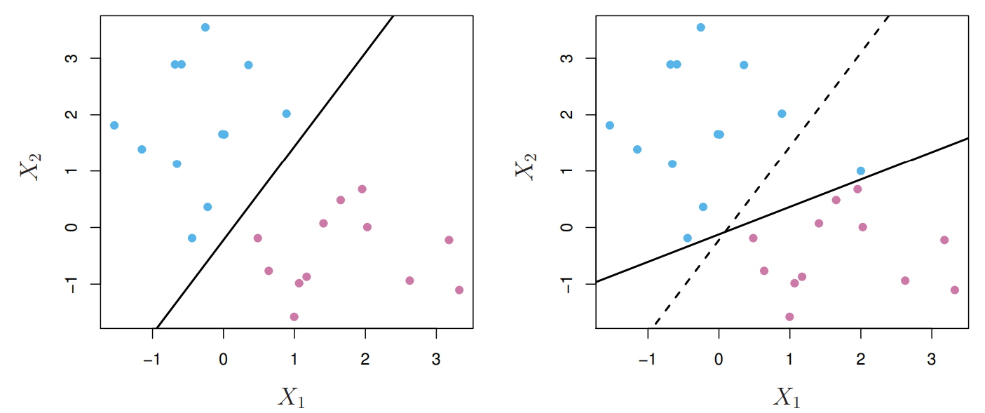
Unfortunately, the MMC suffers from high sensitivity to individual observations. In the figure below, the addition of a single blue observation drastically alters the MMC (left plot original, right plot with additional observation). This is because MMCs perfectly separate all training observations, forcing the MMC to accommodate for observations that may potentially be outliers! This leads to overfitting which reduces MMCs ability to generalize.
The solution to this problem is to allow for misclassification of a few training observations. This tweaks our optimization problem slightly. A nonnegative tuning parameter \(C\) is introduced, which controls the degree of violation allowed. The updated optimization problem is now,
\begin{align}
& \max_{\beta_0,\beta_1,\ldots,\beta_p,\epsilon_1,\ldots,\epsilon_n,M} M \tag{9.12}\\
& \textrm{subject to}\; \sum_{j=1}^p \beta_j^2 = 1 \tag{9.13}\\
& y_i(\beta_0+\beta_1x_{i1}+\beta_2x_{i2}+\ldots+\beta_px_{ip}) \geq M(1-\epsilon_i) \;\; \forall i = 1,\ldots,n \tag{9.14}\\
& \epsilon_i \geq 0, \;\; \sum_{i=1}^n \epsilon_i \leq C \tag{9.15}
\end{align}
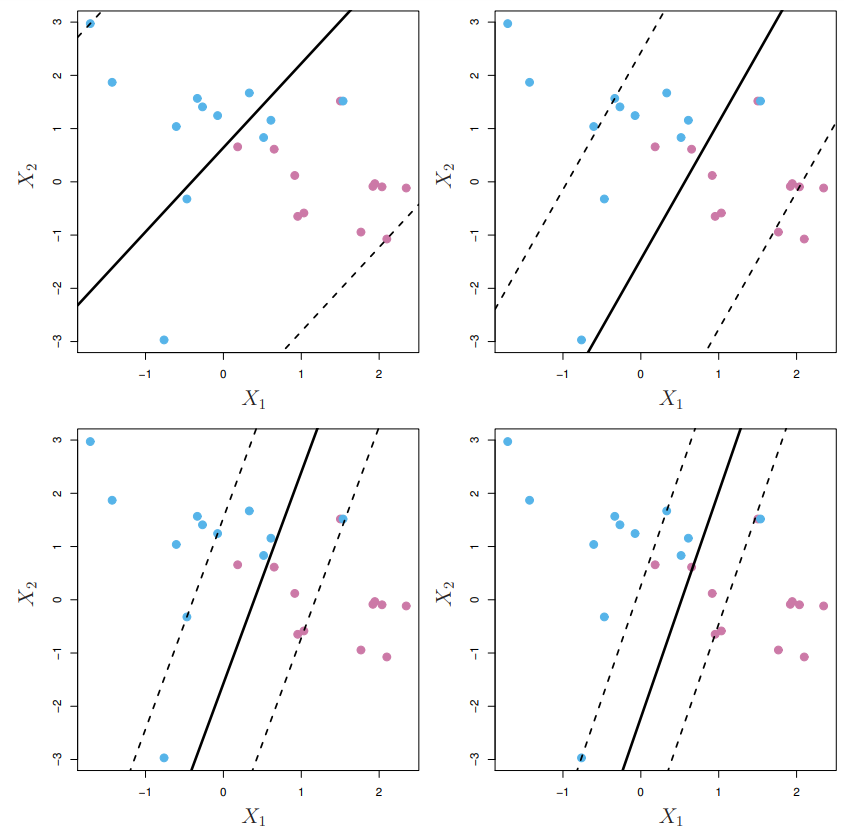
Aside from the new parameter \(C\), we have \(\epsilon_1, \ldots, \epsilon_n\) which tells us where the \(i\)th observation is relative to the hyperplane and margin. In other words, \(\epsilon_i\) tells us how much error we allow for observation \(i\). In this setting, the support vectors are observations which lie directly on the margin, or on the wrong side of the margin. Thus, when \(C\) is large, we actually have more support vectors! The figures below depict how \(C\) influences the SVC. \(C\) is greatest for the top left figure, then top right, bottom left and bottom right. Solid lines represent the hyperplane and the dotted lines describe the margin.
Support Vector Machines
Now we are finally ready to tackle SVMs. In many applications, observations cannot be separated using a linear decision boundary. SVMs circumvent this problem by finding a non-linear decision boundary by expanding the feature space using non-linear kernels. Going back to SVCs, it can be shown that the solution to SVCs only involves inner products between observations (ignore all the math for now). In this case, the inner product is the 'kernel' of the SVC and can be expressed as \(K(x_i,x_{i'})=\sum_{j=1}^p x_{ij}x_{i'j}\). Importantly, the inner product is a linear kernel, which restricts the SVC to only linear decision boundaries. As mentioned before, all the SVM does differently is use non-linear kernels such as,
\begin{align}
K(x_i, x_{i'}) &= (1 + \sum_{j=1}^p x_{ij}x_{i'j})^d\\
K(x_i, x_{i'}) &= exp(-\gamma\sum_{j=1}^p (x_{ij}-x_{i'j})^2)
\end{align}
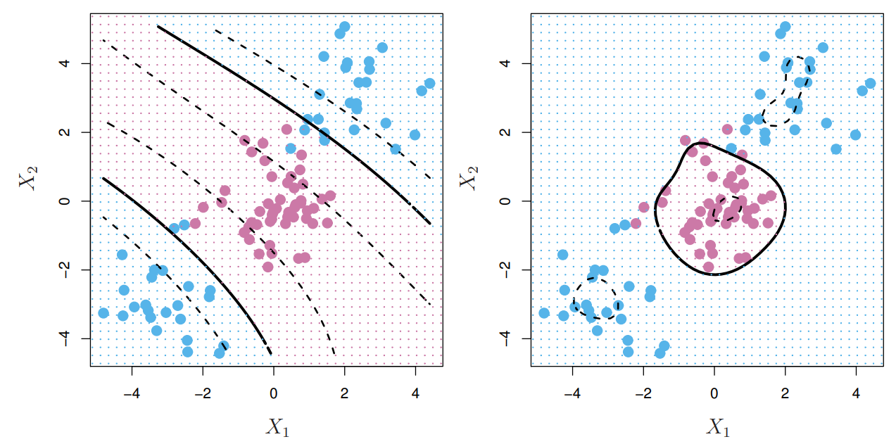
And that’s pretty much it! To wrap up this article on SVMs, here are two figures showing fitted SVMs on datasets where a linear decision boundary would not be effective.
Twitter Facebook LinkedIn

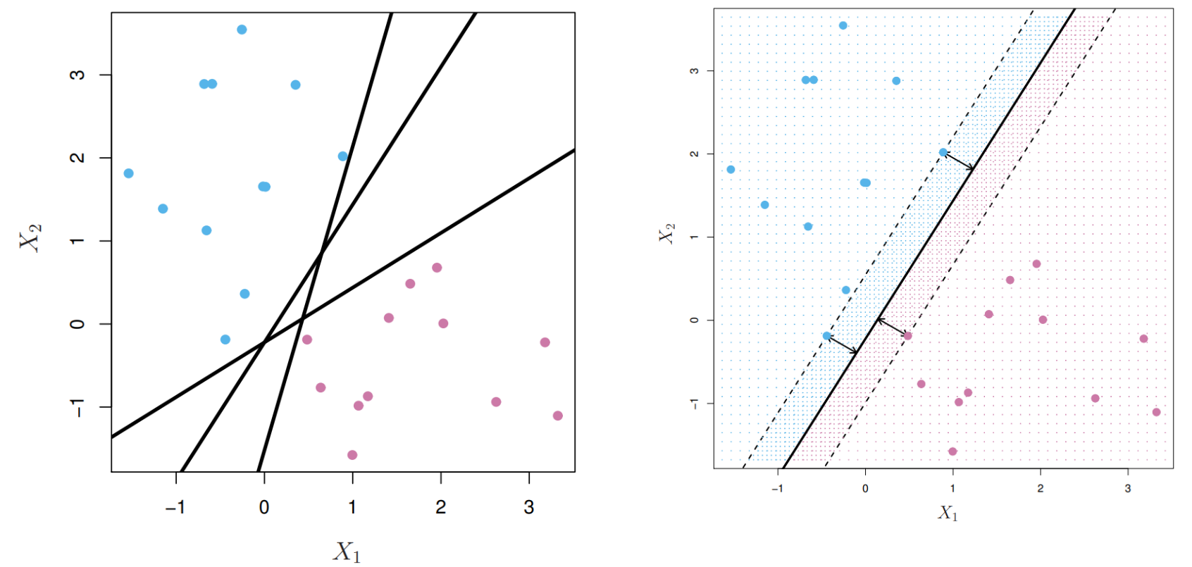 The left plot in the figure above shows three different lines that separate the blue and purple observations. All three do the trick perfectly; no observation is on the wrong side of the line. Which line should we choose then? According to MMC, we should choose the line which maximizes the distance from the closest observations from both classes. These closest observations are called support vectors because they 'support' the hyperplane and are often vectors in high dimensional space. The right plot in the figure denotes the distance between a support vector and the MMC by an arrow and it is clear that the selected line maximizes the distances between support vectors and the line. The optimization problem to solve is as follows where \(y_i \in \{-1, 1\}\),
\begin{align}
& \max_{\beta_0,\beta_1,\ldots,\beta_p,M} M \tag{9.9}\\
& \textrm{subject to}\; \sum_{j=1}^p \beta_j^2 = 1 \tag{9.10}\\
& y_i(\beta_0+\beta_1x_{i1}+\beta_2x_{i2}+\ldots+\beta_px_{ip}) \geq M \;\; \forall i = 1,\ldots,n \tag{9.11}
\end{align}
which can look intimidating at first, but is actually simpler than it looks. Equation 9.11 ensures that each observation lies on the correct side of the hyperplane because \(y_i\) is either -1 or 1 If \(M\) is nonnegative. In conjunction with equation 9.9 the resulting hyperplane will maximize the distance between the hyperplane and the support vectors. Equation 9.10 is primarily for interpretive reasons that we will gloss over for now.
The left plot in the figure above shows three different lines that separate the blue and purple observations. All three do the trick perfectly; no observation is on the wrong side of the line. Which line should we choose then? According to MMC, we should choose the line which maximizes the distance from the closest observations from both classes. These closest observations are called support vectors because they 'support' the hyperplane and are often vectors in high dimensional space. The right plot in the figure denotes the distance between a support vector and the MMC by an arrow and it is clear that the selected line maximizes the distances between support vectors and the line. The optimization problem to solve is as follows where \(y_i \in \{-1, 1\}\),
\begin{align}
& \max_{\beta_0,\beta_1,\ldots,\beta_p,M} M \tag{9.9}\\
& \textrm{subject to}\; \sum_{j=1}^p \beta_j^2 = 1 \tag{9.10}\\
& y_i(\beta_0+\beta_1x_{i1}+\beta_2x_{i2}+\ldots+\beta_px_{ip}) \geq M \;\; \forall i = 1,\ldots,n \tag{9.11}
\end{align}
which can look intimidating at first, but is actually simpler than it looks. Equation 9.11 ensures that each observation lies on the correct side of the hyperplane because \(y_i\) is either -1 or 1 If \(M\) is nonnegative. In conjunction with equation 9.9 the resulting hyperplane will maximize the distance between the hyperplane and the support vectors. Equation 9.10 is primarily for interpretive reasons that we will gloss over for now.
 The solution to this problem is to allow for misclassification of a few training observations. This tweaks our optimization problem slightly. A nonnegative tuning parameter \(C\) is introduced, which controls the degree of violation allowed. The updated optimization problem is now,
\begin{align}
& \max_{\beta_0,\beta_1,\ldots,\beta_p,\epsilon_1,\ldots,\epsilon_n,M} M \tag{9.12}\\
& \textrm{subject to}\; \sum_{j=1}^p \beta_j^2 = 1 \tag{9.13}\\
& y_i(\beta_0+\beta_1x_{i1}+\beta_2x_{i2}+\ldots+\beta_px_{ip}) \geq M(1-\epsilon_i) \;\; \forall i = 1,\ldots,n \tag{9.14}\\
& \epsilon_i \geq 0, \;\; \sum_{i=1}^n \epsilon_i \leq C \tag{9.15}
\end{align}
Aside from the new parameter \(C\), we have \(\epsilon_1, \ldots, \epsilon_n\) which tells us where the \(i\)th observation is relative to the hyperplane and margin. In other words, \(\epsilon_i\) tells us how much error we allow for observation \(i\). In this setting, the support vectors are observations which lie directly on the margin, or on the wrong side of the margin. Thus, when \(C\) is large, we actually have more support vectors! The figures below depict how \(C\) influences the SVC. \(C\) is greatest for the top left figure, then top right, bottom left and bottom right. Solid lines represent the hyperplane and the dotted lines describe the margin.
The solution to this problem is to allow for misclassification of a few training observations. This tweaks our optimization problem slightly. A nonnegative tuning parameter \(C\) is introduced, which controls the degree of violation allowed. The updated optimization problem is now,
\begin{align}
& \max_{\beta_0,\beta_1,\ldots,\beta_p,\epsilon_1,\ldots,\epsilon_n,M} M \tag{9.12}\\
& \textrm{subject to}\; \sum_{j=1}^p \beta_j^2 = 1 \tag{9.13}\\
& y_i(\beta_0+\beta_1x_{i1}+\beta_2x_{i2}+\ldots+\beta_px_{ip}) \geq M(1-\epsilon_i) \;\; \forall i = 1,\ldots,n \tag{9.14}\\
& \epsilon_i \geq 0, \;\; \sum_{i=1}^n \epsilon_i \leq C \tag{9.15}
\end{align}
Aside from the new parameter \(C\), we have \(\epsilon_1, \ldots, \epsilon_n\) which tells us where the \(i\)th observation is relative to the hyperplane and margin. In other words, \(\epsilon_i\) tells us how much error we allow for observation \(i\). In this setting, the support vectors are observations which lie directly on the margin, or on the wrong side of the margin. Thus, when \(C\) is large, we actually have more support vectors! The figures below depict how \(C\) influences the SVC. \(C\) is greatest for the top left figure, then top right, bottom left and bottom right. Solid lines represent the hyperplane and the dotted lines describe the margin.